This is a post about my project on modeling the popularity of online news articles.
The work uses the dataset from the Online News Popularity project that collected data from articles published on Mashable, between January 7 2013 to January 7 2015. The data was the basis for research which resulted in the publication of a paper on “A Proactive Intelligent Decision Support System for Predicting the Popularity of Online News”
The data is mostly clean but there was some work required to combine columns, that were essentially “One Hot Encoded”, into Categorical columns for Data Channel and Day of the Week data as well some scripting to fill in some missing Data Channel values. The main reason for this is that while One Hot Encoding is good for linear models, the tree based models perform better with Ordinal Encoding for Categorical data.
Since the same dataset was used in the Unit1 Build Project, all of this cleanup work was already completed and described in “The Dataset” section of Studying Online News Popularity
The original data cleanup code was used to create CleanupOnlineNewsPopularity.ipynb which stored the cleaned up dataset in a CSV file that was zipped and stored at OnlineNewsPopularity.csv.zip - this was then used as the dataset for this project.
The code for this project is available at OnlineNewsPopularity.ipynb.
A blog post on this work has been published as an article on Medium - Modeling Online News Popularity.
The Dataset
The compressed CSV file was loaded into a Pandas dataframe, initial observations of the dataset revealed that it is a large dataset with 39644 observations of 2 non-predictive(url, timedelta), 47 predictive attributes and 1 target attribute (shares == the number of views for the article).
The problem was changed to one of Classification by creating a new target attribute (popularity == 1 if shares > median/1400 else 0) with 2 classes, popular(1) and unpopular(0). The distribution of popularity values was reasonably balanced with 53% popular(1) and 47% unpopular(0).
The url, timedelta and shares attributes were then dropped from the dataset.
Data Modeling
Since the distribution of popularity values is balanced, accuracy makes a good evaluation metric with the baseline accuracy value being the percentage of the largest class, expressed as a fraction i.e. the baseline accuracy for the entire dataset would be 0.53.
Partitioning
The X dataframe was created by dropping the target(popularity) attribute and the y vector was created from the target attribute column.
Since the dataset is large, sklearn.model_selection.train_test_split was used twice to split it into X_train/y_train(64%:25372), X_val/y_val(16%:6343) and X_test/y_test(20%:7929) datasets.
The baseline accuracy measures for the Training, Validation and Test datasets are 0.54, 0.53 and 0.52 respectively.
Linear Model - Logistic Regression(LogisticRegression with SelectKBest)
For the Linear Model, the data was transformed by using OneHotEncoder() and then scaled using StandardScaler().
The get_best_k_model() function defined below was used to compute the best k, along with the associated features and LogisticRegression() model.
We get a best k value of 51 and the best model has an accuracy of 0.66 against the Validation dataset.
# For parameter k, use SelectKBest to compute the k best
# features and use those to train a LogisticRegressionCV
# model.
def select_and_fit(k, X_tr, y_tr, X_v, y_v):

  selector = SelectKBest(score_func=f_classif, k=k)
  X_train_selected = selector.fit_transform(X_tr, y_train)
  X_val_selected = selector.transform(X_v)

  model = LogisticRegression()
  model.fit(X_train_selected, y_tr)

  return model.score(X_val_selected, y_v), model, selector

def get_best_k_model(X_tr, y_tr, X_v, y_v):
  best_model = None
  best_selector = None
  best_features=[]
  best_k = 0
  best_acc = 0

  # n = 62
  n = X_tr.shape[1]
  # Loop through k and compare accuracies to determine the best
  # k features(best_features) with the highest accuracy
  # One run with k from 1 - 62(range(1,n+1)) gave the best k as 51 - in order to reduce
  # the time looking for best k, we just run once with k=51
  #for k in range(1, n+1):
  for k in range(51, 52):
      acc, model, selector = select_and_fit(k, X_tr, y_tr, X_v, y_v)
      #print(acc, feat)
      if acc > best_acc:
        best_acc = acc
        best_k = k
        best_model = model
        best_selector = selector

  print(f'best_k = {best_k}\nbest Accuracy = {best_acc:0.2f}\n')
Evaluation Metrics
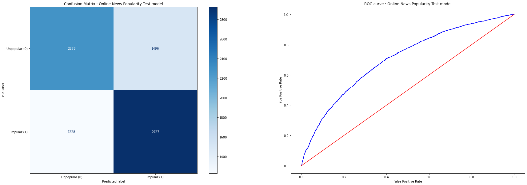
Using the best model gives us the following accuracy/auc scores for the Training, Validation and Test datasets:
| Dataset | Accuracy | Baseline | AUC |
|---|---|---|---|
| Training | 0.66 | 0.54 | 0.71 |
| Validation | 0.66 | 0.53 | 0.71 |
| Test | 0.66 | 0.52 | 0.71 |
Here’re the Confusion Matrix and ROC curves for the Test dataset
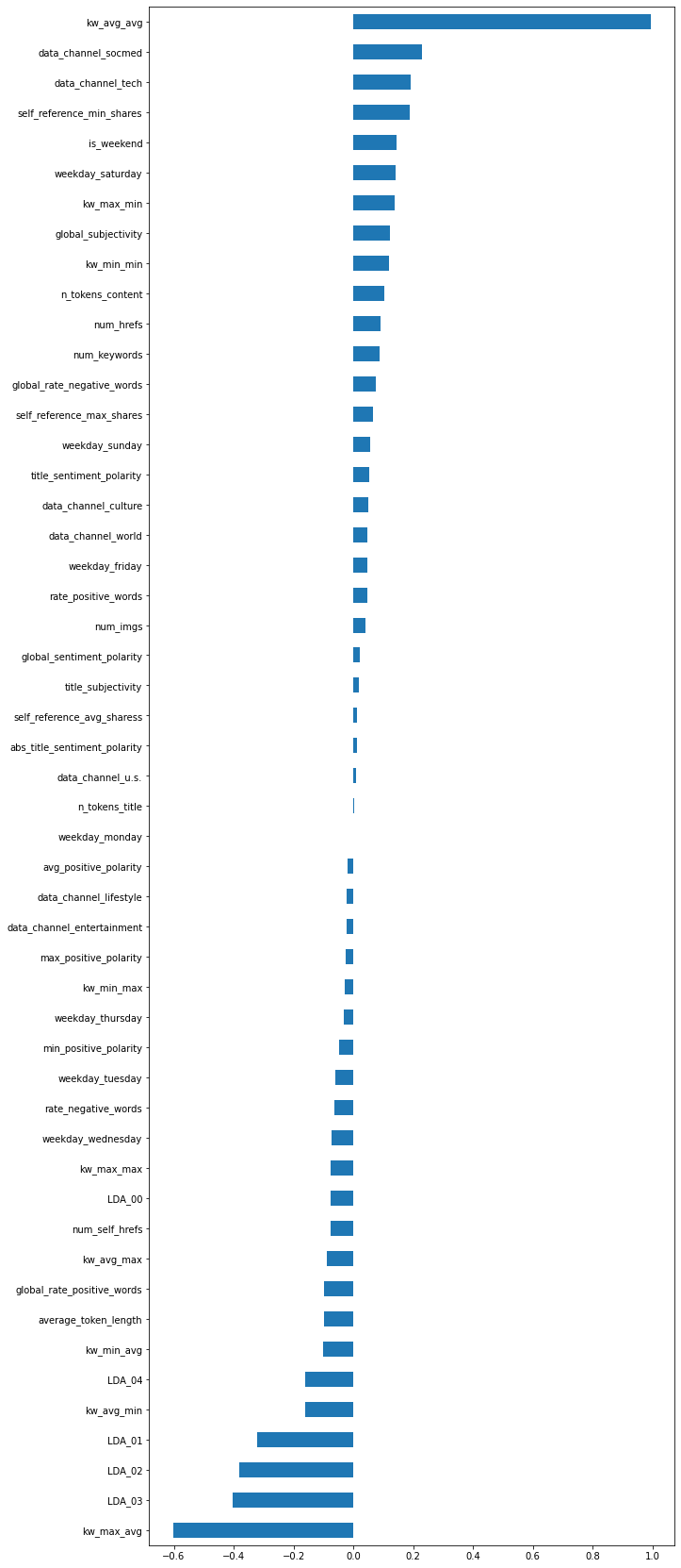
Understanding the Model
Here’s a visualization of the coefficients associated with the 51 features used for the model.
Tree Based Model - Decision Tree(DecisionTreeClassifier)
For the Decision Tree model, the categorical data was encoded using OrdinalEncoder() and the max_depth hyperparameter for the DecisionTreeClassifier() was tuned to 7 using the Validation dataset.
model = make_pipeline(
  OrdinalEncoder(),
  DecisionTreeClassifier(max_depth=7, random_state=42)
)
Evaluation Metrics
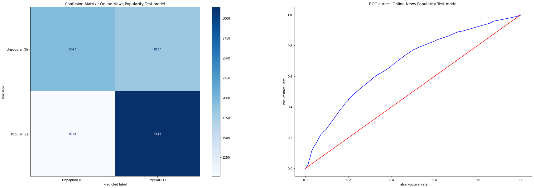
The Decision Tree model gives us the following accuracy/auc scores for the Training, Validation and Test datasets:
| Dataset | Accuracy | Baseline | AUC |
|---|---|---|---|
| Training | 0.67 | 0.54 | 0.73 |
| Validation | 0.64 | 0.53 | 0.69 |
| Test | 0.64 | 0.52 | 0.68 |
Here’re the Confusion Matrix and ROC curves for the Test dataset
Tree Based Model - Random Forest(RandomForestClassifier)
For the Random Forest model, the OridinalEncoder() was used again for the categorical features and the model hyperparameters were tuned to the values shown below using the Validation dataset:
rf_model = RandomForestClassifier(n_estimators=103, random_state=42, n_jobs=-1, max_depth=25, min_samples_leaf=3, max_features=0.3)
Evaluation Metrics
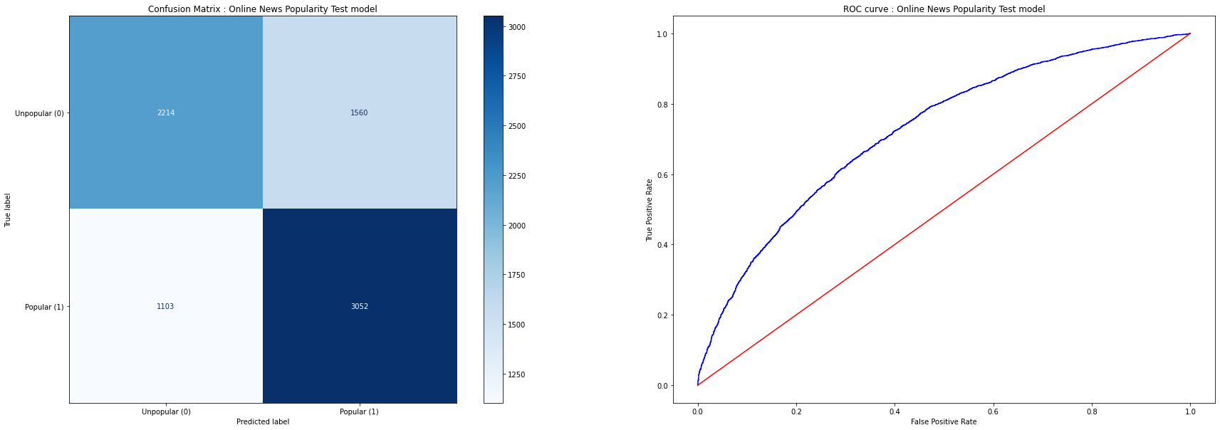
The Random Forest model gives us the following accuracy/auc scores for the Training, Validation and Test datasets:
| Dataset | Accuracy | Baseline | AUC |
|---|---|---|---|
| Training | 1.00 | 0.54 | 1.00 |
| Validation | 0.67 | 0.53 | 0.73 |
| Test | 0.66 | 0.52 | 0.72 |
Here’re the Confusion Matrix and ROC curves for the Test dataset
Understanding the Model
The following table details the importance, computing using PermutationImportance(), of the various features used in the model
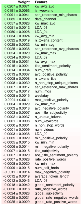
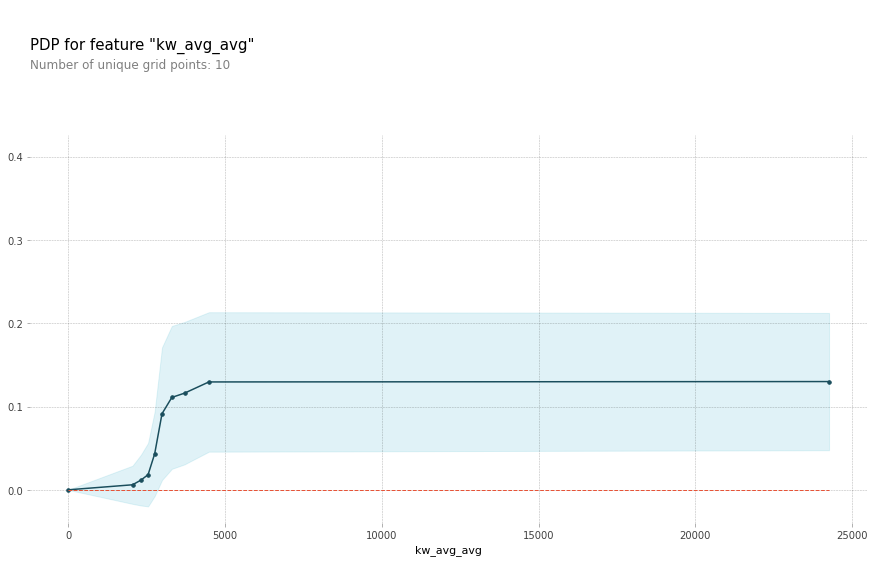
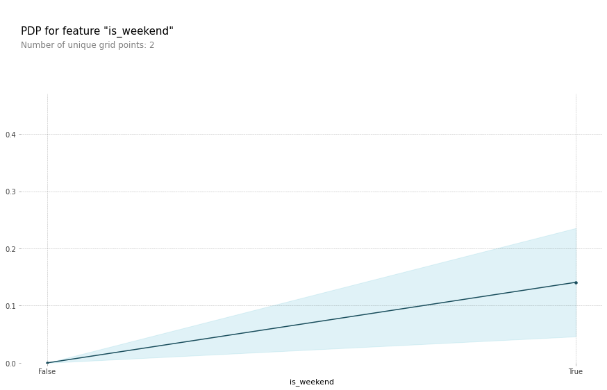
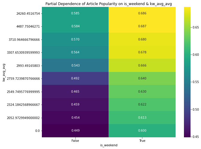
Since the 2 most important features were kw_avg_avg and is_weekend, here’re the Partial Dependence Plots for
kw_avg_avg in isolation:
is_weekend in isolation:
kw_avg_avg, is_weekend interacting:
To get a better understanding of the impact of various features on predictions, here’re SHAP (SHapley Additive exPlanations) plots of
an entry accurately predicted as popular(1)

and
one accurately predicted as unpopular(0)

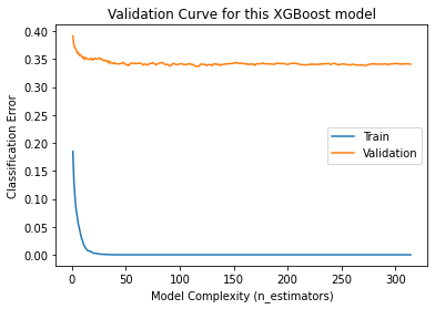
Tree Based Model - Gradient Boosting(XGBoost)
For the Random Forest model, the OridinalEncoder() was used again for the categorical features and the model hyperparameters were tuned as shown below using the Validation dataset:
xgb_model = XGBClassifier(n_estimators=1000, random_state=42, n_jobs=-1, max_depth=13, learning_rate=0.3)
The model was then fit using the 'error' eval metric, generating the best model at iteration 114 and stopping after 314 iterations.
eval_set = [(X_train_encoded, y_train),
            (X_val_encoded, y_val)]

eval_metric = 'error'
xgb_model.fit(X_train_encoded, y_train,
          eval_set=eval_set,
          eval_metric=eval_metric,
          early_stopping_rounds=200)
Here’s the resulting Validation Curve:
Evaluation Metrics
The Gradient Boosting model gives us the following accuracy/auc scores for the Training, Validation and Test datasets:
| Dataset | Accuracy | Baseline | AUC |
|---|---|---|---|
| Training | 1.00 | 0.54 | 1.00 |
| Validation | 0.66 | 0.53 | 0.72 |
| Test | 0.65 | 0.52 | 0.71 |
Here’re the Confusion Matrix and ROC curves for the Test dataset

Conclusion
The Random Forest model exhibited the best behavior, closely followed by Gradient Boosting and Linear models with the Decision Tree model trailing behind.
| Model | Accuracy | AUC |
|---|---|---|
| Random Forest | 1.00/0.67/0.66 | 1.00/0.73/0.72 |
| Gradient Boost | 1.00/0.66/0.65 | 1.00/0.72/0.71 |
| Linear | 0.66/0.66/0.66 | 0.71/0.71/0.71 |
| Decision Tree | 0.67/0.64/0.64 | 0.73/0.69/0.68 |