This is a post about my project on the dataset from the Online News Popularity project that collected data from articles published on Mashable, between January 7 2013 to January 7 2015. The data was the basis for research which resulted in the publication of a paper on “A Proactive Intelligent Decision Support System for Predicting the Popularity of Online News”
The initial focus of the analysis was to examine the effect of removing outliers on the accuracy of Linear Regression models, where accuracy is measured by computing the Mean Absolute Error(MAE).
Once that was done, the focus of the analysis was to partition the dataset into low, medium and high popularity articles and examine, for each partition, the
-
correlation matrices for differences/similarities
-
relationship between the type of article and popularity
-
relationship between the day of the week the article was published and popularity
The code for this project is available at DS-Unit-1-BuildProject.ipynb.
A blog post on this work has been published as an article on Medium - Studying Online News Popularity.
The Dataset
The dataset is contained in a csv file that was packaged into a zip file along with the associated names file describing the dataset. If the csv file were the only file in the zip package, Pandas’ read_csv method could be used to extract the data set.
However, the presence of the additional names file made that impossible and it was necessary to use the io and zipfile packages to get the file readable by read_csv.
onp_url = 'https://github.com/nsriniva/DS-Unit-1-Build/blob/master/OnlineNewsPopularity.zip?raw=true'

# Open the zip file
zfile = urlopen(onp_url)

# Create an IO stream
zfile_mem = io.BytesIO(zfile.read())

# Extract data file from archive and load into dataframe
# The zip archive contains the data file
# OnlineNewsPopularity/OnlineNewsPopularity.csv
# and the info file
# OnlineNewsPopularity/OnlineNewsPopularity.names.
# Use the zipfile package to open the archive and read the data file
with zipfile.ZipFile(zfile_mem) as zf:
  with zf.open('OnlineNewsPopularity/OnlineNewsPopularity.csv') as f:
    onp_df = pd.read_csv(f)
Once loaded into a Pandas dataframe, initial observations of the dataset revealed that it is a large dataset with 39644 observations of 58 predictive attributes and 1 target attribute shares(the number of views for the article).
Some assembly required - processing the data
The datachannel(type of article) and weekday(day of the week on which the article was published) attributes looked interesting and examining their relationship or lack thereof with the popularity of the article appeared to be a good idea. One problem was with the form in which this data was stored in the dataframe - one column/attribute for each datachannel and weekday. The first step was to transform the multiple attributes/columns into a single one for datachannel and weekday.
# First, identify all the data_channel_is_*/weekday_is_* columns
data_channel_columns = list(filter(lambda x: x.startswith('data_channel_is_'), onp_df.columns))
weekday_columns = list(filter(lambda x: x.startswith('weekday_is_'), onp_df.columns))
['data_channel_is_lifestyle',
 'data_channel_is_entertainment',
 'data_channel_is_bus',
 'data_channel_is_socmed',
 'data_channel_is_tech',
 'data_channel_is_world']

['weekday_is_monday',
 'weekday_is_tuesday',
 'weekday_is_wednesday',
 'weekday_is_thursday',
 'weekday_is_friday',
 'weekday_is_saturday',
 'weekday_is_sunday']
Merging the data from the multiple data_channel_is_*/weekday_is_* columns into a single data_channel/weekday was easily achieved. However examining the resultant columns revealed a problem.
display(onp_merged_df.data_channel.value_counts())
display(onp_merged_df.weekday.value_counts())
6    8427
5    7346
2    7057
3    6258
0    6134
4    2323
1    2099
Name: data_channel, dtype: int64
3    7435
2    7390
4    7267
1    6661
5    5701
7    2737
6    2453
Name: weekday, dtype: int64
The data_channel attribute values have the following mappings
OrderedDict([('misc', 0),
             ('lifestyle', 1),
             ('entertainment', 2),
             ('bus', 3),
             ('socmed', 4),
             ('tech', 5),
             ('world', 6)])
While the weekday column has good data for every row, it looks like 6134 entries do not have valid data_channel information. That’s a lot of missing information so something that needed to be rectified, if possible.
Missing data - BeautifulSoup to the rescue
Manually inspected a few of the urls with missing data_channel information and found that the data channel information was encoded in the data-channel attribute of the hgroup element.
<hgroup class="channel page-header post-head" data-channel="entertainment" data-section="sec0=entertainment&sec1=index&sec2=">
<h2>Entertainment</h2>
...
...
...
</hgroup>
Once the information was located, it was a simple matter of using the requests and BeautifulSoup packages to extract it for all the entries that had missing data_channel information.
def get_data_channel(url):
    global dcm_vals_next
    hgroup = BeautifulSoup(requests.get(url).content,'html.parser').find('hgroup')
    ret = 0
    if hgroup is not None:
        dc = hgroup['data-channel']
        if dc not in dcm_keys:
            dcm[dc] = dcm_vals_next
            dcm_keys.append(dc)
            dcm_vals_next += 1
        ret = dcm[dc]
    return ret
The url and data_channel columns were written out to data_channel_df.csv, processed using data_channel_cleanup.py and the new data_channel info was written out to data_channel_cleaned_df.csv
The new data_channel info was merged into the onp_merged_df dataframe and the data_channel column data was examined.
display(onp_merged_df.data_channel.value_counts())
6    9513
2    8384
5    8219
3    6980
4    2323
1    2099
7    1917
8     138
9      46
0      25
Name: data_channel, dtype: int64
Three new data_channel types have been added resulting in a new mapping
OrderedDict([('misc', 0),
             ('lifestyle', 1),
             ('entertainment', 2),
             ('bus', 3),
             ('socmed', 4),
             ('tech', 5),
             ('world', 6),
             ('culture', 7),
             ('u.s.', 8),
             ('social-good', 9)])
Unfortunately, we’re still left with a few(25) entries with no data_channel information.
At this stage, the data has been sufficiently cleaned and is ready for the next step.
Data Analysis
Partitioning
The zscore() method from the scipy.stats package was used to compute z scores for the shares values. These z scores were compared against the specified value to generate a boolean filter array that could be used to paritition the dataset.
def get_outliers_filter(sigma=3):
  z = np.abs(stats.zscore(onp_df.shares))
  return np.where(z>sigma)[0]
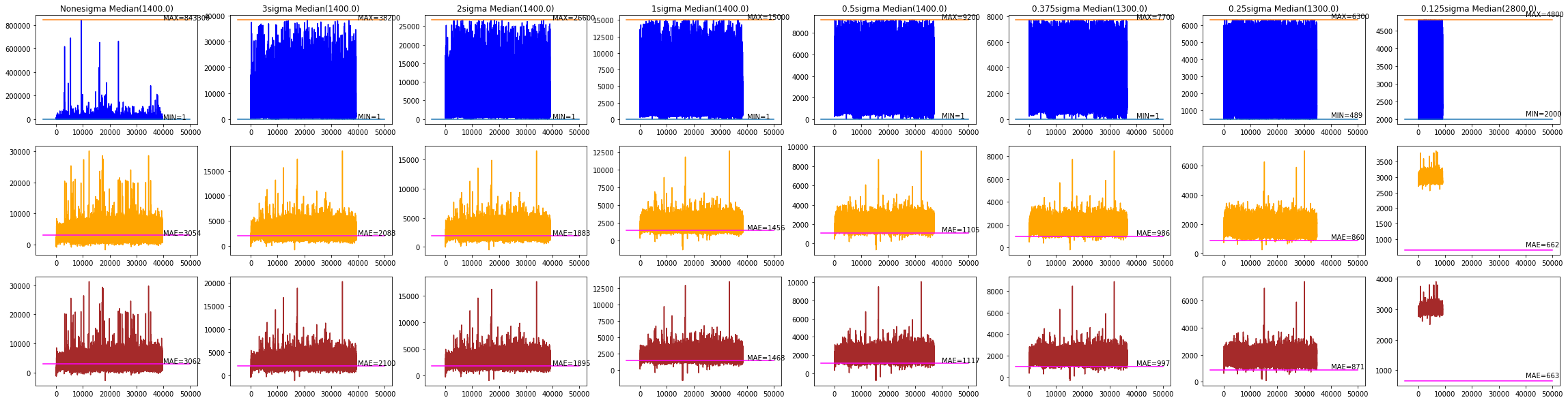
Linear Regression and removing outliers
The LinearRegression() tool from the sklearn.linear_model package was used to generate linear regression models whose accuracy was measured by computing the MAE(Mean Absolute Error).
#Let's try some linear regression
def linear_regression(df, outliers= None):
  if outliers is None:
    X = df.values
    Y = onp_df.shares.values.reshape(-1,1)
  else:
    X = df.drop(outliers).reindex().values
    Y = onp_df.drop(outliers).reindex().shares.values.reshape(-1,1)

  lr = LinearRegression()
  lr.fit(X,Y)
  Yc = lr.predict(X)

  error = Y-Yc

  num = len(Y)

  # Mean absolute error
  mae = np.abs(error).sum()/num
  # Mean square error
  mse = np.linalg.norm(error)/num**0.5

  return num, mae, mse, len(X), Y, Yc
This was performed against the full dataset as well as multiple partitioning scenarios, with the best accuracy(lowest MAE) achieved with a paritioning where both the lower and upper outliers were removed.
Partitioning the dataset and Popularity
For the rest of the analysis, a partitioning was chosen because that was the highest
value where the median(1400) and high(9200) values were both the same order of magnitude.
pop_df, hpop_df = partition_on_shares(onp_merged_df, 0.5)

pop_df_grouped = pop_df.groupby(pop_df.popular)

lpop_df = pop_df_grouped.get_group(0)
mpop_df = pop_df_grouped.get_group(1)
The entries with shares values exceeding were extracted into the hpop_df(high popularity dataframe), with the remaining entries were split into lpop_df(low popularity dataframe) and mpop_df(medium popularity dataframe) datasets based on whether their shares values were < or >= 1400(the median value), respectively.
Correlation Matrix
The seaborn.heatmap was used to display the pairwise correlation of columns computed using the pandas.DataFrame.corr() method against the low, medium and high popularity dataframes.
def display_corr(df, ax,sfx='Low'):
## heatmeap to see the correlation between features.
# Generate a mask for the upper triangle (taken from seaborn example gallery)
  df_corr = df.corr()

  mask = np.zeros_like(df_corr, dtype=np.bool)
  mask[np.triu_indices_from(mask)] = True

  sns.heatmap(df_corr,
              annot=False,
              mask = mask,
              cmap = 'RdBu_r',
              linewidths=0.1,
              linecolor='white',
              vmax = .9,
              ax = ax,
              square=True)

  ax.text(1, 1,f'min({df.shares.min()}) max({df.shares.max()}) num({len(df.shares)})', fontsize='x-large')
  ax.set_title(f'Correlations Among Features in the {sfx} Popularity Range', y = 1.03,fontsize = 20);
The correlation maps for the low/med/high popularity dataframes show distinctively different “signatures”, with surprising similarities between the low and high popularity datasets.
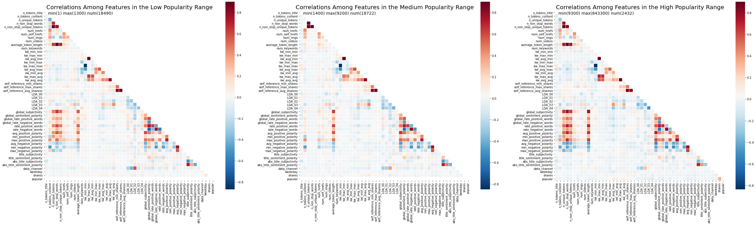
A quick and dirty comparitive summary:
- All 3 datasets appear to be very similar “along the diagonal”
- The data_channel vs LDA_00, LDA_01, LDA_02 correlations are the strongest in the low popularity , reducing in the medium and reducing again in the high popularity dataset.
- The average_token_length vs global_subjectivity, rate_positive_words, avg_positive_polarity, max_positive_polarity, average_negative_polarity, min_negative_polarity correlations are weakest in the low popularity , strengthening in the medium and strengthening again in the high popularity dataset.
- The n_unique_tokens, n_non_stop_words, n_non_stop_unique_tokens vs global_subjectivity, global_rate_positive_words, rate_positive_words, avg_positive_polarity, max_positive_polarity, average_negative_polarity, min_negative_polarity correlations essentially only exist in the low and high popularity datasets but much stronger in the high popularity dataset.
Data Channel Type/Popularity
For this analysis, bar graphs of the percentage of articles per data channel were plotted.
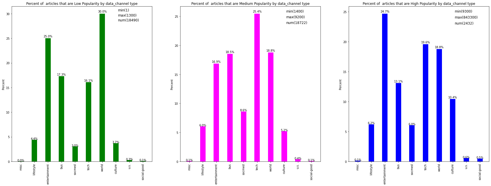
Comparitive Summary:
-
The top 4 channels in each of the low, medium and high popularity datasets are world, tech, entertainment and business
-
A clear winner in the medium popularity dataset are tech articles, with world and bus practically neck and neck for second place with entertainment trailing behind.
-
In the high popularity dataset, entertainment articles are a clear winner, with tech a little behind for second, world not far behind at third and bus a clear laggard.
Weekday/Popularity
For this analysis, bar graphs of the percentage of articles per data channel were plotted.
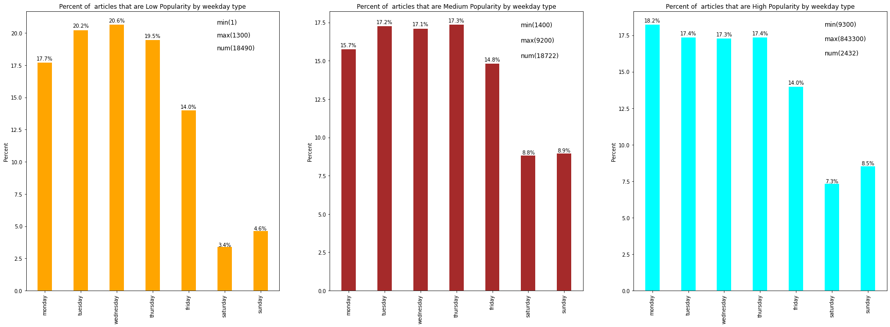
Comparitive Summary:
- Most articles in all 3 datasets were published during the work week.
- For both the medium and high popularity datasets, the number of articles on Tue/Wed/Thu were practically the same with a significant drop on Fri.
- The weekends were better for both the medium and high popularity datasets, as compared to the low popularity i.e. an article published on the weekend(especially Sunday) has a better chance of achieving medium or high popularity.